
Convolutional Neural Nets
I first thought of building a convolutional neural net (CNN) after growing curious about using code to work on something visually-oriented. I’ve always had a strong leaning towards visual aesthetics in my technical work, often enjoying the formatting of dashboards and powerpoint slides more than most normal, sane people. Scanning diagrams of convolutional neural net architecture and becoming intrigued by their ability to analyze images, I thought I’d try my hand.
I spent a week and a half learning about neural nets and then built my own CNN to classify the fashion MNIST dataset, a widely-used collection of 60,000 images of articles of clothing. This post will synthesize what I learned regarding what CNNs are and how they work, while my code implementing the actual model is here. Off we go.
Convolutional neural nets first came about in 2012, when Alex Krizhevsky - a graduate student at the University of Toronto - entered the ImageNet competition (aka the Olympics of computer vision). His model was able to reduce the error record from 26% to 15%, an impressive improvement at the time. His algorithm sparked the revolution of deep learning, a subset of machine learning that uses a layered structure of algorithms called artificial neural networks. As implied by their name, these networks are inspired by the biological neural networks of the human brain. While neural nets are designed to recognize all kinds of patterns, one of the most common use cases is image processing - which is where convolutional neural networks come in. To explain the concept, I’ll take a bird’s eye view - first from 1000 feet, then 100, then 10.
1000-foot bird’s eye view:
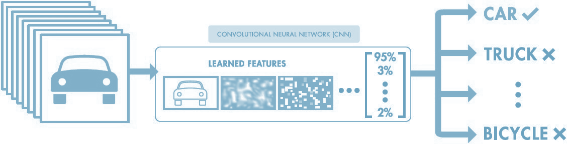
In the general sense, a CNN is a model that takes an input image, passes it through different kinds of filters to extract certain features from the image (ears, whiskers, paws), then uses these extracted features to classify the image into a corresponding label (cat). The CNN is able to capture spatial and temporal dependencies within an image to “see the bigger picture”, using its knowledge of the combination of certain features to develop a holistic understanding of the image contents.
100-foot bird’s eye view:
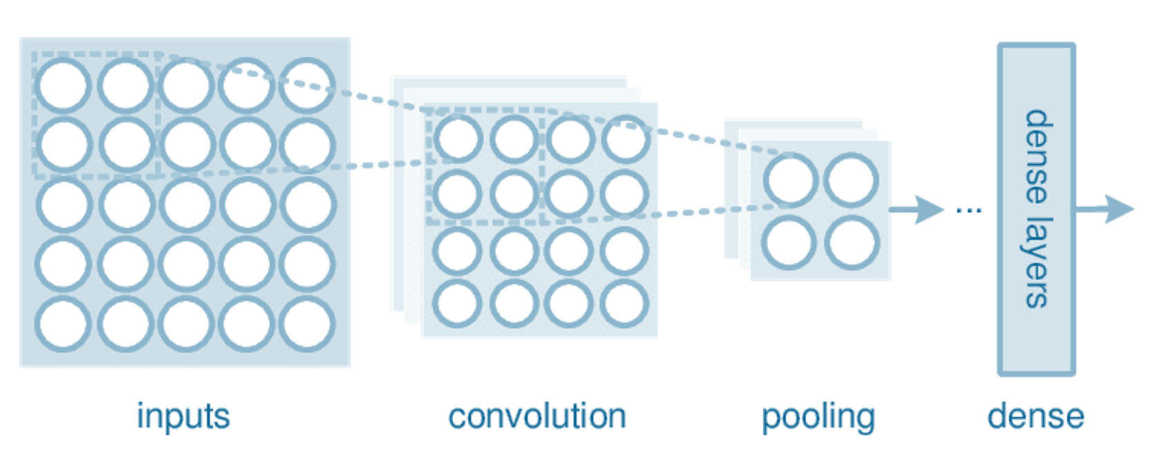
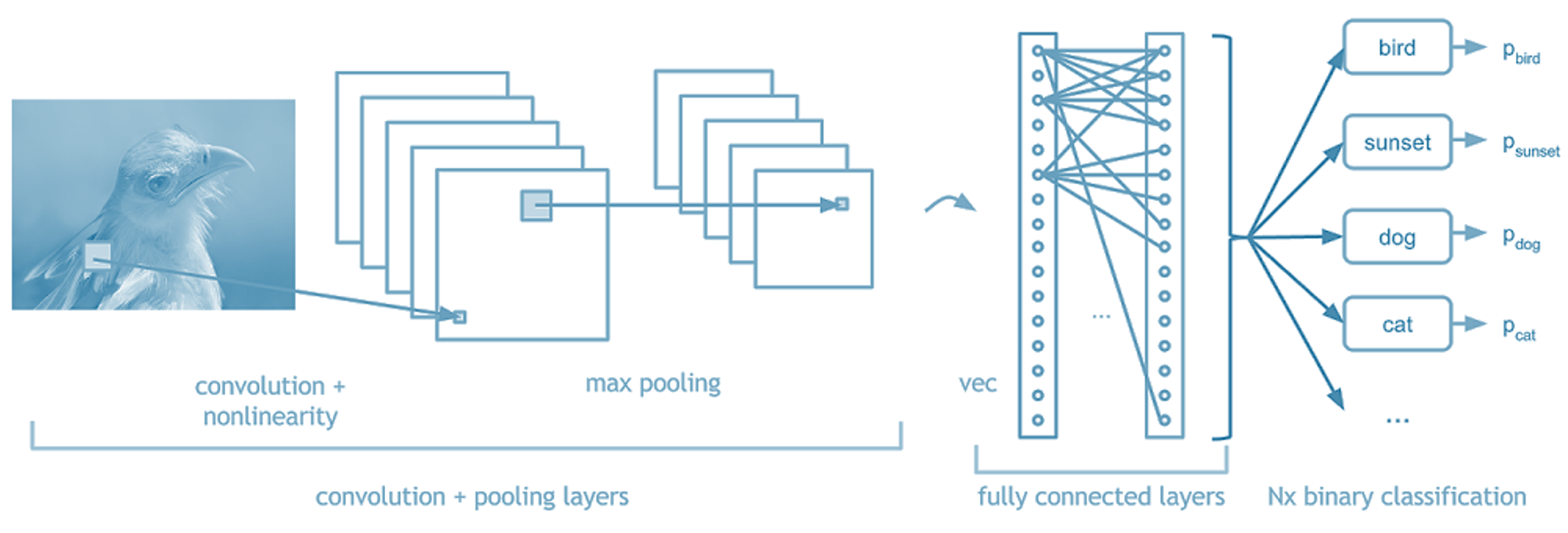
Model architecture: Like other neural nets, convolutional neural nets are made up of hidden layers; each of these layers serve a different purpose in the model. Layers can be added to the model like legos - the more layers, the more complex the model. All CNNs are made up of a combination of four layer types; convolutional layers, pooling layers, dropout layers, and fully connected layers.
Inputs: input images are fed to the model by converting their colors to numbers. Since each pixel in an image is one color, and each color can be represented by a numeric value, we can reduce a 2-D image to a matrix that the computer can then use for mathematical calculations.
Convolutional Layer: What makes a convolutional neural network different from other kinds of neural nets is the inclusion of convolutional layers, which is where feature extraction (the magic) happens. Each convolutional layer consists of filters that “look” for certain shapes and features in the image, resulting in a new, filtered image called a feature map.
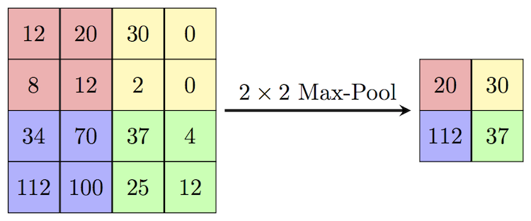
Pooling Layer: Pooling layers reduce the size of the preceding feature maps in order to reduce the computational burden of data processing. They “pool” pixels together by using just the maximum or the average of a group of pixels as the new output. The principle here is that we can simplify the images by dropping out insignificant details while retaining the important stuff, like whether and where a feature exists.
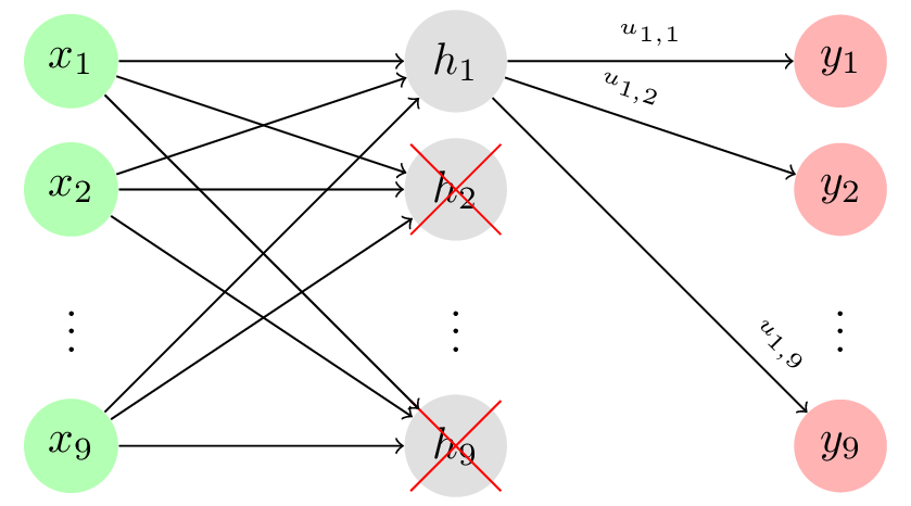
Dropout Layer: Each value in the new image after it has been processed by a convolutional or pooling layer is called a neuron. Dropout layers drop a random set of these neurons by setting them equal to zero, forcing the model to learn to classify images on less than 100% of the data. By preventing the model from growing too dependent on the training dataset, dropout layers improve the model’s ability to correctly categorize unseen data, reducing the risk of overfitting.
Fully Connected Layer: After detecting features, we use a fully connected layer (also called a dense layer) to the end of the network. This layer looks at the feature maps and determines which combinations of features correspond to each class. For example, a fully connected layer would combine the knowledge of the existence of whiskers, four legs, and triangular ears to classify an image as a cat.
Backpropagation: You may be wondering how the filters in a model know to look for these features, and how the fully connected layer knows what combinations of features to look at. Through a process called backpropagation, the computer trains the model by adjusting filter weights until it minimizes the error in the final prediction. Similarly to how we don’t know the difference between a cat or a dog when we were born, but later learn the names for each creature as we are given their corresponding labels, the filter weights in a CNN are initially randomized and then updated to detect the most useful features over time.
10-foot bird’s eye view:
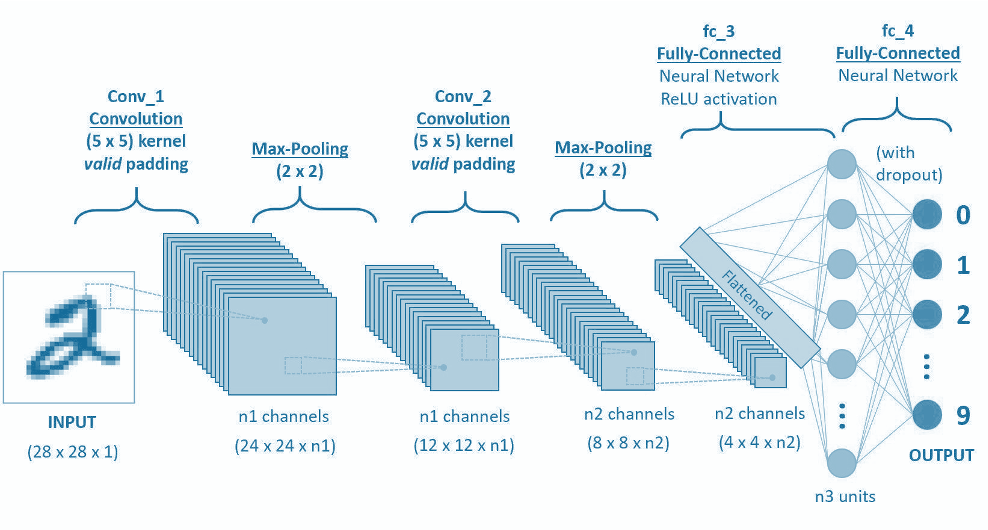
Let’s walk through the architecture of a simple convolutional neural net in more detail, roughly represented in the image below.
Input:
As mentioned above, input images are converted to matrices where each value in the matrix corresponds to the color value in that pixel. A grayscale 28x28 image is converted to a 28x28x1 matrix, where the 1 corresponds to the “depth” of the picture. A color 28x28 image is converted to a 28x28x3 matrix, as each pixel’s color is expressed as a combination of reds, greens, and blues (RGB). For the explanation below, we’ll assume we’re working with grayscale images.
Convolutional Layer:
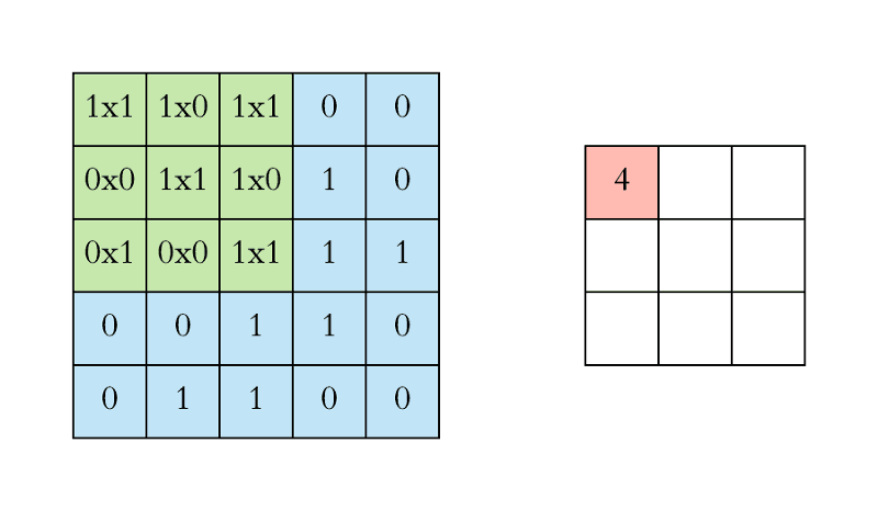
The convolutional layer is the core lego of a convolutional neural network; it does the heavy-lifting in understanding the contents of the images. In our first convolutional layer, let’s say we have 4 filters that each have a size of 5x5 pixels. Each of these 5x5 filters detects a different feature by multiplying the filter values by values in the input image. More specifically, we take the dot product of the filter (hi, linear algebra class from 2348 years ago) with corresponding regions in the input image. This sliding of the filter along the width and height of the input is called “convolving”. This resulting feature map is a new, filtered image with greater values where a feature was detected, and smaller values in the absence of a feature. In the image below, we have a 5x5 pixel input image and a 3x3 filter with values [[1,0,1],[0,1,0],[1,0,1]]. We convolve the filter (in green) across every region in the image (blue) to get a new representation of the image (pink).
After every convolution operation, we apply an activation function to transform the summed weighted input into an output to be fed (or not fed, depending on the output value itself) to the next layer. The default activation function for convolutional neural networks is the rectified linear activation function, or ReLU, which is a piecewise linear function that outputs the input directly if positive, otherwise zero. This value - the original number itself, or zero - is then propagated to the next layer. Just as certain neurons fire in the brain when receiving a stimulus, this function determines whether that neuron is fired and its value sent as input to the next layer, essentially deciding whether a feature is “present enough” to be considered.
Pooling Layer:
In taking just one input image and convolving 4 filters around the image, we end up with 4 new feature maps that are new versions of the original image with certain features extracted. You can imagine that with thousands of images and multiple convolutional layers, the amount of parameters and computation in the network will quickly grow very large. To reduce this and control for overfitting, it’s common practice to insert a pooling layer between successive convolutional layers. These pooling layers reduce the dimensions of the images by taking the maximum (max-pooling) or the average (average-pooling) of each nxn region in the preceding layer’s output. Many models use a 2x2 maxpool layer with a stride of 2, meaning the layer takes the maximum of a 2x2 region in the image and then slides right or down by 2 pixels - effectively halving the width and height of the original matrix. By reducing the dimensions in this way, we preserve important information while reducing the size of the image and thus the computation time for subsequent layers.
Dropout Layer:
While pooling layers reduce the dimensions of the image by using a metric - maximum or average - to “summarize” certain regions, dropout layers simply set certain neurons to zero ito prevent over-fitting. Neurons are randomly dropped with probability p, forcing the network to learn robust features that are not overly dependent on the features of the training dataset.
Fully Connected Layer:
Our last layer - the fully-connected layer, also called a dense layer. This layer takes the knowledge we now have about the features in our input images and returns the probability that the image belongs to a certain class. While convolutional and pooling layers identify individual characteristics in the images, the dense layer combines these characteristics together to better understand the bigger picture (get it??? ok sorry). In this layer, we use a function called the softmax activation function to calculate the probability that each image belongs to a certain class.
All of the above happens in passing a batch of training samples through the model in a process called forward propagation. For each batch we calculate the error at the output layer - or how “off” our model was - and then use backpropagation to adjust the parameters in each layer to minimize the error. This adjustment is done through gradient descent, in which weights are adjusted in proportion to their contribution of the total error.
Finally, when a new, unseen image is fed into our trained model, the network will output probabilities for each class; the interpretation of the model’s ultimate “decision” is whichever class has the highest calculated probability. If the training set was large enough and our model was built with parameters that adequately capture image features without overfitting, the network will hopefully generalize well to new pictures and classify them correctly.
There’s a lot this post doesn’t talk about, like some more detailed model parameters (padding and stride, bias, data augmentation) and how to actually tune the parameters in the model. For me, though, this process of self-teaching a concept, implementing it in code, then synthesizing my learnings in writing has been a fun exercise in being a beginner again. The CNN I built to classify the fashion MNIST dataset was ultimately 92% accurate in its predictions - but much of this high accuracy is due to the structure of the dataset itself, so I won’t flatter myself. More fun problems and projects to come.
Image Sources (as they appear):